Problem and prerequisites
A fast average algorithm does not prove that every part receives a timely decision. Measure the whole path under concurrent camera, processing and storage load, using the station’s actual decision deadline.
Prepare the test
Assume sequential capture 10 ms, transfer 20 ms, queue 15 ms, processing 70 ms and output 5 ms: 120 ms total against a 200 ms deadline, leaving 80 ms illustrative reserve. This is a planning sum, not a benchmark; real stages may overlap.
Define the operational deadline and its measurement boundaries before quoting a processing time. A line may need the final output before a physical reject point, while a robot may need a validated target before issuing motion. Specify whether latency starts at the physical trigger, host request or exposure start, and ends at computation, transmitted result or observed output. Those are different measurements. Record the hardware, camera formats, acquisition rates, algorithm or model, application version and output path used in the test. Include the planned number of cameras and image-retention policy. Warm-up and startup behavior should be identified explicitly so that a fast steady-state run does not conceal a slow first production request.
Procedure
- Define start and finish events and their clock domains; never subtract unsynchronized device timestamps.
- Use a monotonic clock for host intervals and verified synchronization or external measurements across devices.
- Run 1000 planned cycles with all cameras and intended image retention active; retain each part identifier and stage times.
- Add slow storage and peak traffic separately, then together; count missing and late results, not only completed fast ones.
- Test timeout handling so a missed deadline produces the agreed fault or disposition instead of an old pass.
Timestamp acquisition, transfer completion, processing-queue entry, processing start and final output wherever the implementation permits reliable observation. Use monotonic host time for host intervals. Relate device clocks to that timeline through a validated method or use external measurement for physical trigger-to-output timing. Treat a timestamp stamped when the application notices an event as a received-event time, not automatically as the hardware’s occurrence time. Load all planned cameras, normal communication and image writing concurrently. Introduce a slow consumer and the expected burst pattern, then observe queue depth and age as well as completion time. Keep missing triggers, rejected requests and acquisition faults in the run ledger rather than dropping them from the dataset.
Illustrative test record
Illustrative assumptions, not measured Deyi performance. Replace these values with your own signed test records.
| Record | Assumed value |
|---|---|
| Capture and analysis interval | 10 ms |
| Transfer interval | 20 ms |
| Processing interval | 70 ms |
| Decision deadline | 200 ms |
For each scheduled trigger, record whether it completed, exceeded the deadline or never produced a result. Compute latency percentiles from completed results, but report missing and late counts alongside them; omitting failures makes the distribution misleading. Load image writing and all planned cameras concurrently, then introduce a slow consumer. A 120 ms illustrative sum does not establish the maximum observed latency, and a 1000-cycle run cannot establish a rare-failure rate.
The illustrative stage sum is a worksheet, not a benchmark. Sequential durations add to 120 ms and leave an arithmetic 80 ms against the assumed deadline. Actual stages may overlap or queue, so measure end-to-end intervals directly and explain how the internal stage times relate to them. Report the tested load, completed count, late count, missing count, latency distribution and worst observed value. Percentiles describe only the population used to calculate them; a low percentile does not authorize excluding failed requests. Check whether long latency coincides with network transfer, consumer backlog, algorithm work or file writing before changing a setting. A resource correlation suggests the next controlled experiment, not proof of the cause.
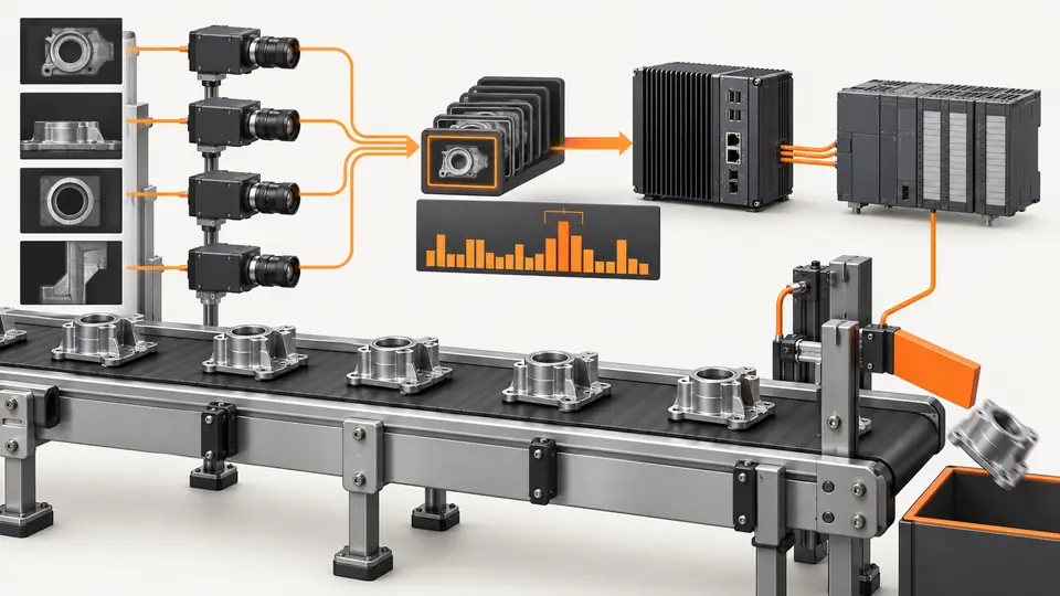
Two views of the workflow
Load-test latency from trigger to PLC decision — 1
The measured path includes capture, transfer, waiting, analysis and output. Assign timestamps at boundaries rather than guessing from frame rate.
- Capture
- Transfer
- Queue and process
- PLC result
Load-test latency from trigger to PLC decision — 2
An idle test, full-load test and fault-injection test answer different questions; keep their results separate.
- Idle load
- Production load
- Injected fault
Troubleshooting
- Large queue time indicates contention or insufficient consumer capacity.
- Transfer spikes require examining stream statistics and network load.
- Clock jumps or negative durations invalidate timing evidence until the measurement method is corrected.
Acceptance and handover
Accept against agreed deadline, missing-result and fault-handling requirements. Report observed maximum and test conditions without promising untested tail behavior. Recheck after changes to camera count, pixel format, algorithm or retention; 1000 cycles alone do not establish long-term reliability.
Set acceptance limits before testing and retain the original evidence. The examples here do not establish a supplied model’s capabilities.
Acceptance requires meeting the agreed timing and disposition rules under representative maximum planned load, including the defined startup and recovery cases. Repeat after the proposed change with the same workload and an unchanged baseline comparison. Verify that reducing queue depth or dropping frames does not create an apparently faster result by losing required inspections. Confirm that late decisions remain bound to their original part and receive the specified containment response. Retain configuration, clock method, event ledger and traces so another reviewer can reproduce the calculation. A 1000-cycle trial can expose functional and load problems, but cannot establish the probability of a rare failure over long production. Handover should state tested conditions and exclusions, without promoting the example’s 120 ms into a guaranteed supplied-system latency.
Sources and technical references
These references explain the methods and limits used in this tutorial. Example checks are guidance; production acceptance requires evidence from your own samples.
- Acquisition Timing InformationBasler
Distinguishes acquisition stages and model-specific timing limits.
Checked - Optimizing GigE Vision Systems in pylonBasler
NIC, packet timing, bandwidth and stream statistics under single/multi-camera load.
Checked
Component and selection references
- Machine Vision Acceptance Test Checklist
- Smart Camera vs PC-Based Vision System
- Visual Inspection System Design Checklist
- Machine Vision Systems
- machine vision software
- EAN-13 traceability: line acceptance
- EAN-13 traceability: decode and data rules
- Stable camera acquisition: buffers, timeouts and reconnection
- Accept and integrate a visible fill-level workflow
- AI-assisted workflow for a visible level proxy
- Link inspection records, images and part identifiers
- OCR labels: acceptance and PLC contract
- OCR labels: native workflow and exact match
- Accept and integrate open-package completeness checks
- Build an AI-assisted open-package completeness workflow
- Build a PLC–vision handshake with explicit states
- Seal and bead appearance: line acceptance
- Seal and bead appearance: workflow rules
- SKU color sorting: acceptance and unknown route
- SKU color sorting: typed color and SKU rules
- Surface defects: acceptance and line output
- Surface defects: bounded AI evaluation
- Version and roll back the complete vision recipe